How to use NLP to classify tweets

Image by Luke Chesser on Unsplash

Using machine learning to classify tweets about real disasters or not

Over the years, we have seen Twitter evolve from just a social media to also a business and news platform. While this growth is excellent, it has also caused an increase in the spread of fake news which can have serious effects around the world.

This project aims to address the problem of fake news using real disasters. We will use a dataset of tweets and their corresponding labels to train a model that can predict if a tweet reports fake news about disasters or not.

Data

The data was obtained from Kaggle and consists of training data and test data in two separate CSV files. There are 7,613 entries in the training dataset and 3,263 entries in the test dataset.

The training dataset contains [id, location, keyword, text and target] columns. The id column has a unique id for each tweet, location and keyword columns contain the location the tweet was sent from and a particular keyword in the tweet respectively; however, not every row has a value in these two columns. The text column contains the main text with URLs if there was a link in the tweet and the target column is for the label of each tweet. All columns are of string datatype apart from the target column which is an integer.
The test dataset contains the same columns except the target column.

Overview

I trained a Gaussian Naive Bayes, Logistic regression and Gradient boosting classifier for this task. The text column was used as the feature because it is a better representation of a tweet while the target column was used as the label.

Exploratory Data Analysis

For Exploratory Data Analysis (EDA), below is a visualisation of the top ten keywords with the most fake disaster tweets.

import pandas as pd
train_df = pd.read_csv('train.csv')

# Get list of keywords with their count of fake disaster tweets, sort the list in descending order
keywords= [(i, len(train_df[(train_df['keyword']==i) & (train_df['target']==0)])) for i in train_df['keyword'].unique()]
keywords.sort(key = lambda x: x[1], reverse=True)

# Plot bar graph of keywords with the most fake disaster tweets
x, y = (zip(*keywords))

x = [str(i) for i in (x)][:10]
y = [int(i) for i in (y)][:10]

Cleaning and Preprocessing

Regex was used to clean each tweet removing every URL links and other characters apart from alphanumeric characters. The text was left in alphanumeric form because some tweets contained figures which are important. Then the text was preprocessed using Gensim and NLTK, resulting in a tweet being a list of word strings. Preprocessing carried out was lemmatization to reduce words to basic form so they can be analysed as one word irrespective of previous inflections; stemming which gets rids of prefixes and suffixes to reduce words to their root form even if the resulting stem is not a valid word in that language; and tokenization to convert sentences into individual words, known as tokens.

import regex as re
import gensim
from gensim.utils import simple_preprocess
from gensim.parsing.preprocessing import STOPWORDS
from nltk.stem.porter import PorterStemmer
from nltk.stem import WordNetLemmatizer, SnowballStemmer

# Function to preprocess data with Gensim
def preprocess_gensim(text):
    # Remove non-alphanumeric characters from data
    text = [re.sub(r'[^a-zA-Z0-9]', ' ', text) for text in text]

    # Lemmatize, stem and tokenize words in the dataset, removing stopwords
    text = [(PorterStemmer().stem(WordNetLemmatizer().lemmatize(w, pos='v')) )for w in text]
    result = [[token for token in gensim.utils.simple_preprocess(sentence) if not token in 
              gensim.parsing.preprocessing.STOPWORDS and len(token) > 3] for sentence in text]
    return result

When comparing NLTK library to Gensim library for stopwords, I discovered the Gensim stopwords collection was more comprehensive than NLTK’s so I decided to go ahead with Gensim stopwords package.

import nltk
from nltk.corpus import stopwords
import gensim
from gensim.parsing.preprocessing import STOPWORDS

# download list of stopwords (only once; need not run it again)
nltk.download("stopwords")
nltk.download('punkt')
stop_words = set(stopwords.words('english'))

The stemming algorithm used was PorterStemmer.
PorterStemmer and SnowballStemmer give similar results but Porter stemmer is an older algorithm. Its main concern is removing the common endings to words so that they can be resolved to a common form. Typically, it’s not really advised to use the PorterStemmer for any production/complex application; instead, it has its place in research as a nice, basic stemming algorithm that can guarantee reproducibility. It is also said to be gentle when compared to others. However, there is about a 5% difference in the way that Snowball stems versus Porter.¹

Modelling

After each tweet has been preprocessed, we transform them into a Bag-of-Words (BoW) vector. A BoW model is a representation of text that describes the occurrence of words within a document. It is a way of getting features from text without keeping information about the order of words in the document. A BoW is a vector of numbers which each number representing a word in the sentence.
X_train and X_test are the tweets while y_train and y_test are the labels of the respective tweets in the training and test data. train_test_split module splits arrays or matrices into random train and test subsets in the ratio (3:1 unless otherwise specified).

from sklearn.model_selection import train_test_split

#Split data into train and test data
X_train, X_test, y_train, y_test = train_test_split(train_df['text'].to_list(), train_df['target'].to_list(), random_state=0)

# Carry out preprocessing on text data
words_train, words_test = preprocess_gensim(X_train), preprocess_gensim(X_test)

The vocabulary is a set of all words in the training set and is what the supervised learning algorithm is trained based on. Test data is transformed so that the learned model can be applied for prediction in the future.

from sklearn.feature_extraction.text import CountVectorizer

# Extract Bag-of-Words (BoW)
vectorizer = CountVectorizer(preprocessor=lambda x: x, tokenizer=lambda x: x)
features_train = vectorizer.fit_transform(words_train).toarray()

features_test = vectorizer.transform(words_test).toarray()

# Create a vocabulary from the dataset
vocabulary = vectorizer.vocabulary_

Next step is to normalise the BoW feature vectors. This gives each vector a unit length and stop longer tweets (documents) from dominating those with fewer word counts; but, still retaining the unique mixture of feature components.

import sklearn.preprocessing as pr

# Normalize BoW features in training and test set
features_train = pr.normalize(features_train, axis=0)
features_test = pr.normalize(features_test, axis=0)

Algorithms

• Gaussian Naive Bayes Classifier: The first choice was the Gaussian Naive Bayes Classifier. Tree-based algorithms often work quite well on Bag-of-Words as their highly discontinuous and sparse nature is nicely matched by the structure of trees. Ideally, due to better result in both binary and multi-class problems and independence rule, Naive Bayes algorithm has a higher success rate as compared to other algorithms. It assumes that features follow a normal distribution and it is very fast to train. The Gaussian Naive Bayes’ model had a high accuracy score on the train data but did not really perform well on test data. This is known as overfitting which occurs when a model performs very well on training data but struggles to accurately predict test data. It is caused by a model picking up unnecessary noise from the training dataset, learning it and trying to apply them on the test data. Overfitting can be prevented by using cross-validation to fit multiple models on the training data and then comparing their respective performances on unseen data.

• Logistic Regression: Given that the first model did not give a very impressive accuracy score on the test data, I decided to try out by training a logistic regression model. Logistic regression is a discriminative model, as opposed to Naive Bayes that is a generative classifier. In discriminative models, you have “less assumptions” because it learns the posterior probability p(x|y) “directly”. Although Naive Bayes converges quicker, it typically has a higher error than logistic regression. On small datasets, you might want to try out naive Bayes, but as your training set size grows, you likely get better results with logistic regression. The solver is a parameter of the Logistic regression model that dictates which algorithm is used to solve the problem. I went ahead with the default solver, ‘lbfgs’ . It uses multinomial loss algorithm in the optimisation, works best on not-so-large datasets and saves a lot of memory. The maximum number of iterations taken for the solver to converge was set at 1000. After training the logistic regression model, the accuracy score of the model on test data improved.

• Gradient Boosting Algorithm: Gradient boosting builds an additive model in a forward stage-wise fashion; it allows for the optimization of arbitrary differentiable loss functions. Boosting is a sequential technique which works on the principle of ensemble. It combines a set of weak learners and delivers improved prediction accuracy. Unfortunately, this model performed averagely on both train and test data and due to the limited resources, I decided not to pursue it further.

Hyperparameters Tuning

Hyperparameter tuning is the act of searching for the right set of hyperparameters to achieve high precision and accuracy for a model. A hyperparameter is any parameter whose value, if changed, can affect the learning process and performance of the model on the data. The aim is to find a balance between underfitting and overfitting. There are various tuning techniques such as Grid search, Random search, etc. Grid search was the model selection technique used in this project to tune hyperparameters. It loops through predefined hyperparameters and fits the model on the train data. From this, you can select the best parameters for that model. You can also cross-validate each set of hyperparameters multiple times. One drawback of the Grid search is that time complexity explodes with more dimensions and hyperparameters to tune. It suffers from the curse of dimensionality, i.e., the efficiency of the algorithm decreases rapidly as the number of hyperparameters being tuned and the range of values of hyperparameters increase.⁶ It is common to use this technique when the parameters are not more than 4.

• Tuning Gaussian Naive Bayes with var_smoothing: Var_smoothing is a parameter that can be tuned to improve the performance of a Naive Bayes estimator. Its default value is 1e-9 and is of type, float. It is the portion of the largest variance of all features that is added to variances for calculation stability.³ Because Naive Bayes assumes the data follows a normal distribution, it essentially assigns more weights to samples closer to the distribution mean. The variable, var_smoothing, artificially adds a user-defined value to the distribution’s variance (whose default value is derived from the training data set). This essentially widens (or “smooths”) the curve and accounts for more samples that are further away from the distribution mean and helps avoid overfitting. The var_smoothing chosen were 10 samples of evenly spaced numbers between 0 to -9 on a log scale. However, the tuned model’s best score was still not very impressive so I decided to tune the Logistic regression estimator.

from sklearn.model_selection import GridSearchCV
from sklearn.model_selection import RepeatedStratifiedKFold

params_NB = {'var_smoothing': np.logspace(0,-9, num=10)}
cv_method = RepeatedStratifiedKFold(n_splits=2, 
                                    n_repeats=3, 
                                    random_state=0)

gs_NB = GridSearchCV(estimator=nb, 
                     param_grid=params_NB, 
                     cv=cv_method,
                     verbose=1, 
                     scoring='accuracy')

gs_NB.fit(features_train, y_train);

• Tuning Logistic regression with Inverse regularization parameter(C): C is a control variable that retains strength modification of regularization by being inversely positioned to the Lambda regulator. Smaller values specify stronger regularization. “Regularization is any modification we make to a learning algorithm that is intended to reduce its generalization error but not its training error.”⁴ This prevents the algorithm from overfitting the training dataset.
  This tuned estimator performed better than the others on test data.

from scipy.stats import uniform
from sklearn.linear_model import LogisticRegression

logistic = LogisticRegression(solver='saga', tol=1e-2, max_iter=1000, random_state=0)
hyperparameters = dict(C=uniform(loc=0, scale=4), penalty=['l2', 'l1'])
param_grid = {'C': [100, 10, 1.0, 0.1, 0.01]}
k = RepeatedStratifiedKFold(n_splits=2, n_repeats=3, random_state=0)

grid = GridSearchCV(logistic, param_grid=param_grid, cv=k, n_jobs=4, verbose=1)
grid.fit(features_train, y_train)

Evaluation

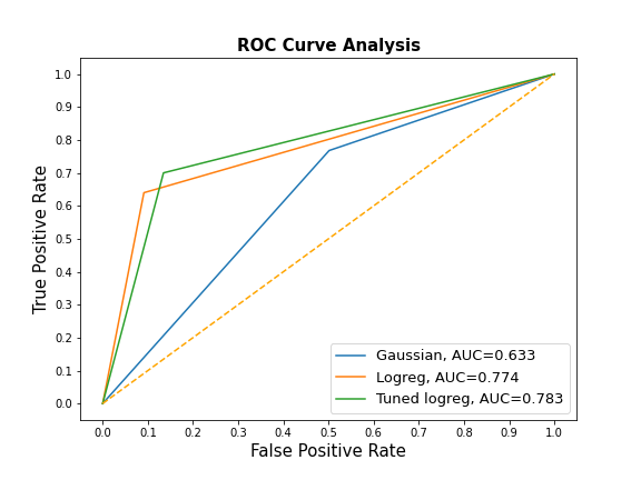
Using the Scikit-learn classification report, I compared metrics across the three main estimators (Gaussian naive Bayes, Logistic Regression and tuned Logistic Regression). Accuracy score and AUROC were also compared. The computed Area Under the Receiver Operating Characteristic Curve (AUROC) shows the performance of a classification model at all classification thresholds from prediction scores.
The Naive Bayes estimator had the highest sensitivity while the tuned Logistic regression has the highest specificity.

from sklearn.metrics import roc_curve

ypreds=[y_pred1, y_pred2, y_pred3]
result_table = pd.DataFrame(columns=['fpr','tpr'])

for pred in ypreds:
    fpr, tpr, _ = roc_curve(y_test, pred)
    auc = roc_auc_score(y_test, pred)
    result_table = result_table.append({'fpr':fpr, 
                                        'tpr':tpr,
                                       'auc': auc},
                                       ignore_index=True)

models = ['Gaussian', 'Logreg', 'Tuned logreg']
result_table['models'] = models
result_table.set_index("models", inplace = True)

fig = plt.figure(figsize=(8,6))

for i in result_table.index:
    plt.plot(result_table.loc[i]['fpr'], 
             result_table.loc[i]['tpr'], 
             label="{}, AUC={:.3f}".format(i, result_table.loc[i]['auc']))

plt.plot([0,1], [0,1], color='orange', linestyle='--')

plt.xticks(np.arange(0.0, 1.1, step=0.1))
plt.xlabel("False Positive Rate", fontsize=15)

plt.yticks(np.arange(0.0, 1.1, step=0.1))
plt.ylabel("True Positive Rate", fontsize=15)

plt.title('ROC Curve Analysis', fontweight='bold', fontsize=15)
plt.legend(prop={'size':13}, loc='lower right')

plt.show()

Conclusion

The tuned Logistic regression model had the highest average precision, recall, accuracy, AUROC score and f1-score so it was selected as the best performing model in this project. However, it is noted that the accuracy score of the model on test data could be improved. This could be by trying out a deep learning algorithm, like Recurrent Neural Network (RNN) to see its performance on the data.

For the full notebook for this article, check out my GitHub repo below: https://github.com/AniekanInyang/tweet-classification

Link to Part 2 of the series where I used Recurrent Neural Network (RNN) to solve the problem: How to use NLP to classify tweets (Part II)

Feel free to reach out on LinkedIn, Twitter or send an email: contactaniekan at gmail dot com if you want to chat about this or any NLP research project.

Stay safe.😷

References

[1] https://towardsdatascience.com/stemming-lemmatization-what-ba782b7c0bd8

[2] https://www.cs.cmu.edu/~tom/mlbook/NBayesLogReg.pdf

[3] https://scikit-learn.org/stable/modules/generated/sklearn.naive_bayes.GaussianNB.html

[4] I. Goodfellow, Y. Bengio, and A Courville, “Deep Learning”, London (2017), The MIT Press.

[5] https://scikit-learn.org/stable/modules/generated/sklearn.metrics.classification_report.html

[6] J. Wiu, X Chen, H. Zhang, L. Xiong, H. Lei and S. Deng, Hyperparameter Optimization for Machine Learning Models Based on Bayesian Optimization (2019), Journal of Electronic Science and Technology.